Generalized Local States Example

This example depicts the basic use of generalized local states in the context of RC as implemented in rescomp.esn.ESNGenLoc()

A more detailed explanation of generalized local states is given here:

Baur, S.; Räth, C. Predicting High-Dimensional Heterogeneous Time Series Employing Generalized Local States. Phys. Rev. Res. 2021, 3, 23215.

import numpy as np
import matplotlib.pyplot as plt
import rescomp
from rescomp.simulations import simulate_trajectory

Simulation Parameters

lor_dim = 40
lor_dt = 0.05
lor_force = 5

shuffle = False
disc_ts = 10000
sync_ts = 2000
train_ts = 100000
pred_ts = 500

tot_ts = disc_ts + 2 * sync_ts + train_ts + pred_ts

Simulation

np.random.seed(1)

starting_point = lor_force * np.ones(lor_dim) + 1e-5 * np.random.rand(lor_dim)
sim_data = rescomp.simulate_trajectory(
        sys_flag='lorenz_96', dt=lor_dt, time_steps=tot_ts,
        starting_point=starting_point, force=lor_force)

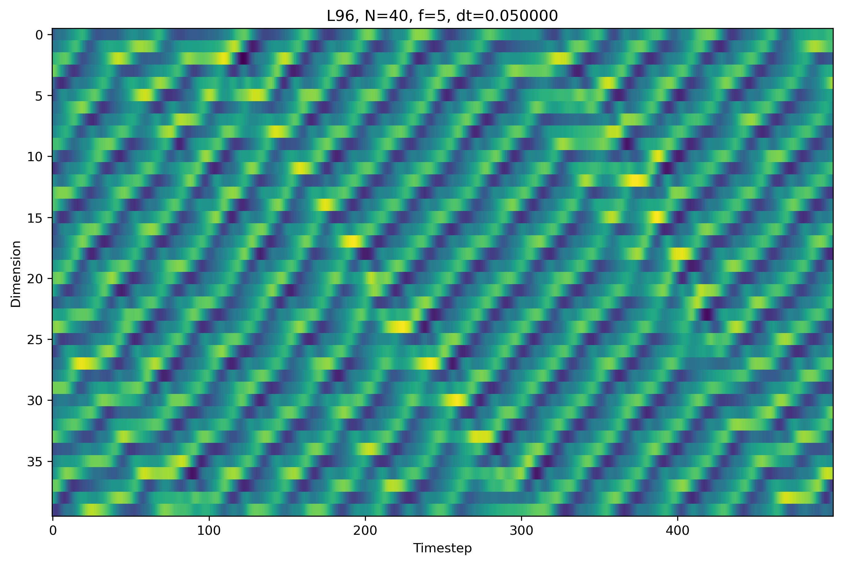
Plot the simulation

lor_title = "L96, N=%d, f=%d, dt=%f"%(lor_dim, lor_force, lor_dt)

lor_axis_ranges = [-pred_ts, tot_ts]

lor_xlabel = "Timestep"
lor_ylabel = "Dimension"

signal_raw = sim_data
y_test = signal_raw[lor_axis_ranges[0]: lor_axis_ranges[1]]

fig, ax = plt.subplots(1, 1, figsize=(9, 6), constrained_layout=True, dpi=300)

vmin = np.min(y_test)
vmax = np.max(y_test)

im = ax.imshow(y_test.T, aspect='auto', vmin=vmin, vmax=vmax)

ax.set_title(lor_title)
ax.set_xlabel(lor_xlabel)
ax.set_ylabel(lor_ylabel)

Text(0, 0.5, 'Dimension')

Add normal noise to the training data. This is not necessary for the generalized local state code to work, but it’s more realistic and increases long term prediction accuracy. Note that we don’t add noise to the data used to test the prediction.

noise_scale = 1e-2

ts_until_train_end = disc_ts + sync_ts + train_ts
noise = np.random.normal(scale=noise_scale, size=[ts_until_train_end, signal_raw.shape[1]])
signal = np.copy(signal_raw)
signal[:noise.shape[0]] = signal[:noise.shape[0]] + noise

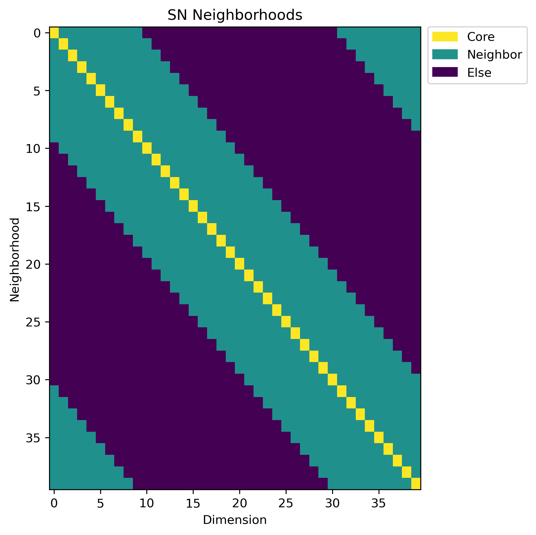
Calculate the different locality matrices, then put them into neighborhoods.

• SN: Spatial neighborhood. Just put the spatially closest dimensions together. Spatial in this case refers to the dimension’s index, so dimension 2 is closer to dimension 3 than it is to dimension 15.

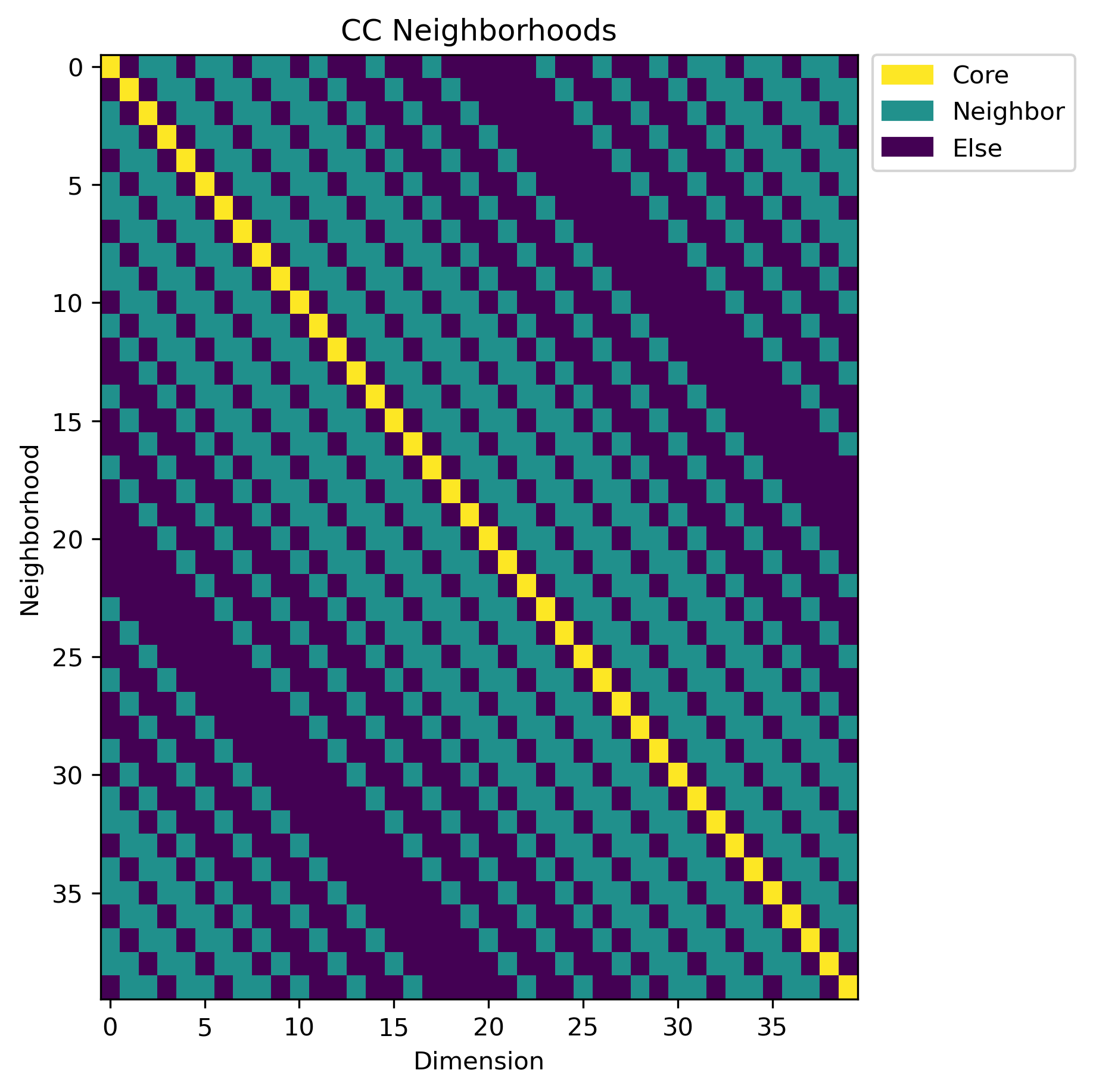
• CC: Cross Correlation Neighborhood. Locality is calculated via the cross correlation between dimensions.

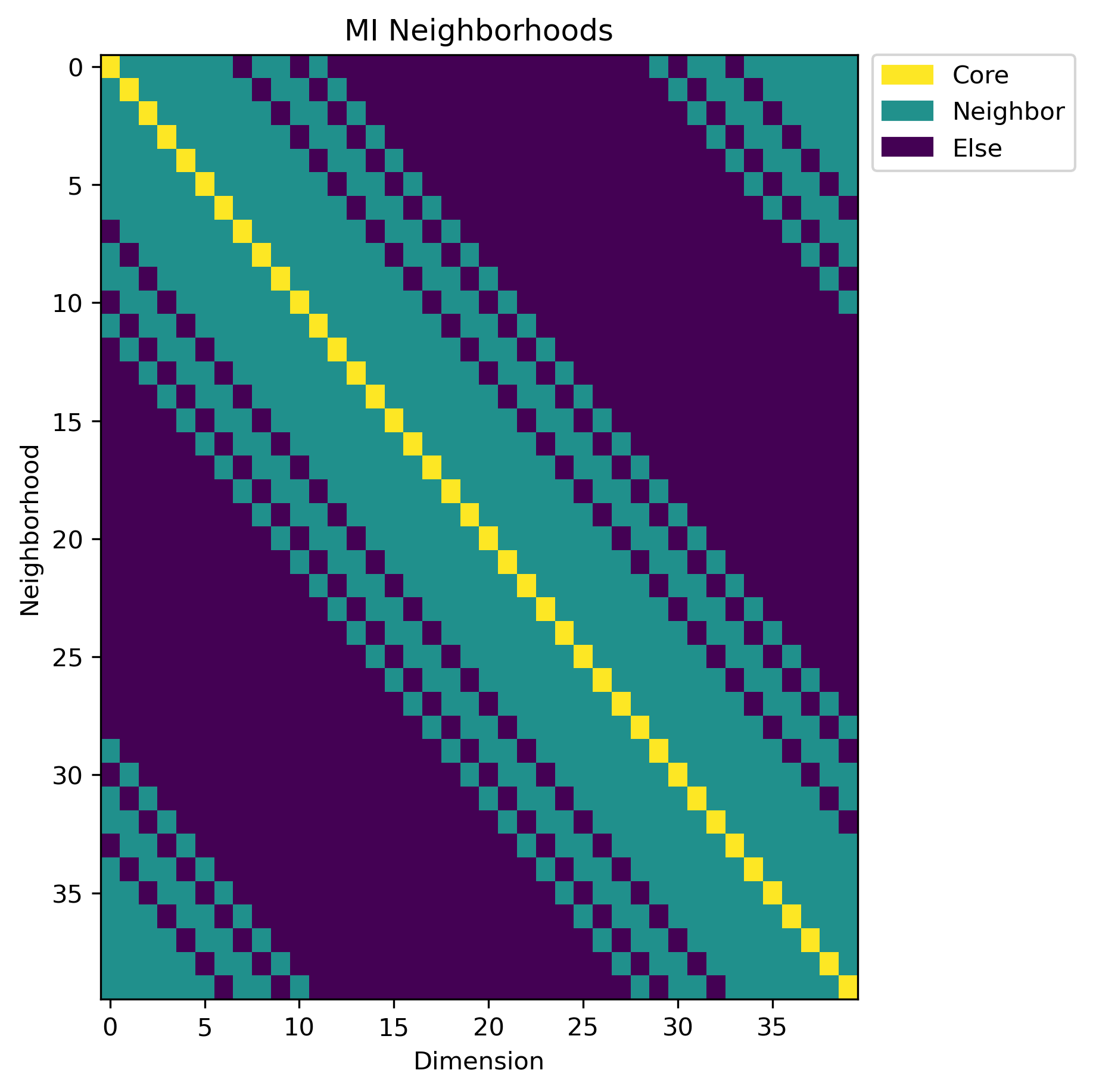
• NMI: (Normalized) Mutual Information Neihborhood. Locality is calculated via via the normalized mutual information between dimensions.

We also set the number of neighbors to 18, simply because it works well for this iteration of the L96 system used as data here.

A larger number of neighbors results in a possibly better prediction at the cost of requiring larger reservoirs and longer training times. Making the neighborhood too small though, will cut out important dimensions, possibly reducing prediction accuracy or making training completely impossible.

If you don’t know your neighborhood size a priori just treat the neighborhood size as another hyperparameter to optimize somewhere in the range of 10 to 50 and you will probably be fine.

For more detail on how the above is implemented exactly, please read Baur, Räth 2021, PRR

sn_loc_matrix = rescomp.locality_measures.sn_loc(signal)
cc_loc_matrix = rescomp.locality_measures.cc_loc(signal)
nmi_loc_matrix = rescomp.locality_measures.nmi_loc(signal)

nbs = 18 # Nr. of neighbors in each neighborhood

sn_nbhds = rescomp.locality_measures.find_local_neighborhoods(
                sn_loc_matrix, neighbors=nbs)
cc_nbhds = rescomp.locality_measures.find_local_neighborhoods(
                cc_loc_matrix, neighbors=nbs)
nmi_nbhds = rescomp.locality_measures.find_local_neighborhoods(
                nmi_loc_matrix, neighbors=nbs)

Define a plotting helper function to make the labels in the plots below look nicer.

import matplotlib.patches as mpatches

def force_colorbar_legend(ax, im, labels, label_values):
    label_colors = [im.cmap(im.norm(value)) for value in label_values]

    patches = [mpatches.Patch(label=labels[i], color=label_colors[i])
               for i in range(len(label_values))]

    ax.legend(handles=patches, bbox_to_anchor=(1.02, 1), loc=2,
              borderaxespad=0.)

Plot the three neighborhoods we calculated above.

For ‘simple’ systems defined by a purely local interaction which is known a priori, as is the case for the L96 system we simulated above, the SN neighborhood is essentially the ‘correct’ neighborhood. That the CC and MI neighborhoods are able to mostly reproduce the SN neighborhood to such a degree is a strong indication that they actually “understood” the relation between the dimensions in this case.

titles = ["SN Neighborhoods", "CC Neighborhoods", "MI Neighborhoods"]
nbhds = [sn_nbhds, cc_nbhds, nmi_nbhds]

for i in range(3):

    fig, ax = plt.subplots(1, 1, figsize=(6, 6), constrained_layout=True, dpi=300)

    im = ax.imshow(nbhds[i], aspect='auto')

    ax.set_title(titles[i])
    ax.set_xlabel("Dimension")
    ax.set_ylabel("Neighborhood")

    labels = ['Core', 'Neighbor', 'Else']
    label_values = [2, 1, 0]

    force_colorbar_legend(ax, im, labels, label_values)

Here we choose the neighborhood to use for the ESN training and prediction below.

Which one to choose, or if you should just calculate/define your own neighborhood separate from the three we defined above, depends on the problem you are trying to solve.

# loc_nbhds = sn_nbhds # Works quite well
# loc_nbhds = cc_nbhds # Doesn't work all that well due to the "nearest neighbors" not being included
loc_nbhds = nmi_nbhds # Works quite well as it's pretty close to the "correct" neighborhood

Create the ESN setup, in this case given by the ESNGenLoc() class. Then train and predict with it, as we have done in the other examples.

As training and prediction will take quite a while (30-60 minutes), we also set the console logger to “debug”, which will print out the calculation process to the terminal.

n_dim = 5000
w_out_fit_flag = "linear_and_square_r"
avg_degree = 3
regularization = 1e-6
spectral_radius = 0.5
w_in_scale = 0.5
w_in_sparse = True
train_core_only = True

loc_esn = rescomp.esn.ESNGenLoc()
loc_esn.set_console_logger("DEBUG")

loc_esn.create_network(n_dim=n_dim,n_rad=spectral_radius, n_avg_deg=avg_degree)

y_pred, y_test = loc_esn.train_and_predict(
    x_data=signal,
    disc_steps=disc_ts,
    train_sync_steps=sync_ts,
    train_steps=train_ts,
    pred_sync_steps=sync_ts,
    loc_nbhds=loc_nbhds,
    reg_param=regularization,
    w_in_scale=w_in_scale,
    w_in_sparse=w_in_sparse,
    train_core_only=train_core_only,
    w_out_fit_flag=w_out_fit_flag
    )

04-05 20:54:23 [DEBUG  ] Start locality training with 40 neighborhoods
04-05 20:54:23 [DEBUG  ] Deepcopy initial ESN instance for each Neighborhood. Reservoir network matrix are shallow copies though.
04-05 20:54:23 [DEBUG  ] Start Training of Neighborhood 1/40
04-05 20:55:25 [DEBUG  ] Start Training of Neighborhood 2/40
04-05 20:56:32 [DEBUG  ] Start Training of Neighborhood 3/40
04-05 20:57:37 [DEBUG  ] Start Training of Neighborhood 4/40
04-05 20:58:42 [DEBUG  ] Start Training of Neighborhood 5/40
04-05 20:59:48 [DEBUG  ] Start Training of Neighborhood 6/40
04-05 21:00:54 [DEBUG  ] Start Training of Neighborhood 7/40
04-05 21:01:59 [DEBUG  ] Start Training of Neighborhood 8/40
04-05 21:03:06 [DEBUG  ] Start Training of Neighborhood 9/40
04-05 21:04:24 [DEBUG  ] Start Training of Neighborhood 10/40
04-05 21:05:30 [DEBUG  ] Start Training of Neighborhood 11/40
04-05 21:06:35 [DEBUG  ] Start Training of Neighborhood 12/40
04-05 21:07:40 [DEBUG  ] Start Training of Neighborhood 13/40
04-05 21:08:46 [DEBUG  ] Start Training of Neighborhood 14/40
04-05 21:09:52 [DEBUG  ] Start Training of Neighborhood 15/40
04-05 21:11:08 [DEBUG  ] Start Training of Neighborhood 16/40
04-05 21:12:14 [DEBUG  ] Start Training of Neighborhood 17/40
04-05 21:13:20 [DEBUG  ] Start Training of Neighborhood 18/40
04-05 21:14:37 [DEBUG  ] Start Training of Neighborhood 19/40
04-05 21:15:42 [DEBUG  ] Start Training of Neighborhood 20/40
04-05 21:16:46 [DEBUG  ] Start Training of Neighborhood 21/40
04-05 21:18:04 [DEBUG  ] Start Training of Neighborhood 22/40
04-05 21:19:09 [DEBUG  ] Start Training of Neighborhood 23/40
04-05 21:20:15 [DEBUG  ] Start Training of Neighborhood 24/40
04-05 21:21:21 [DEBUG  ] Start Training of Neighborhood 25/40
04-05 21:22:40 [DEBUG  ] Start Training of Neighborhood 26/40
04-05 21:23:45 [DEBUG  ] Start Training of Neighborhood 27/40
04-05 21:24:51 [DEBUG  ] Start Training of Neighborhood 28/40
04-05 21:26:08 [DEBUG  ] Start Training of Neighborhood 29/40
04-05 21:27:14 [DEBUG  ] Start Training of Neighborhood 30/40
04-05 21:28:19 [DEBUG  ] Start Training of Neighborhood 31/40
04-05 21:29:24 [DEBUG  ] Start Training of Neighborhood 32/40
04-05 21:30:41 [DEBUG  ] Start Training of Neighborhood 33/40
04-05 21:31:47 [DEBUG  ] Start Training of Neighborhood 34/40
04-05 21:32:52 [DEBUG  ] Start Training of Neighborhood 35/40
04-05 21:34:09 [DEBUG  ] Start Training of Neighborhood 36/40
04-05 21:35:14 [DEBUG  ] Start Training of Neighborhood 37/40
04-05 21:36:20 [DEBUG  ] Start Training of Neighborhood 38/40
04-05 21:37:26 [DEBUG  ] Start Training of Neighborhood 39/40
04-05 21:38:42 [DEBUG  ] Start Training of Neighborhood 40/40
04-05 21:39:48 [DEBUG  ] Start local prediction
04-05 21:39:48 [DEBUG  ] Start syncing
04-05 21:40:01 [DEBUG  ] Prediction for 0/500 steps done
04-05 21:40:04 [DEBUG  ] Prediction for 500/500 steps done

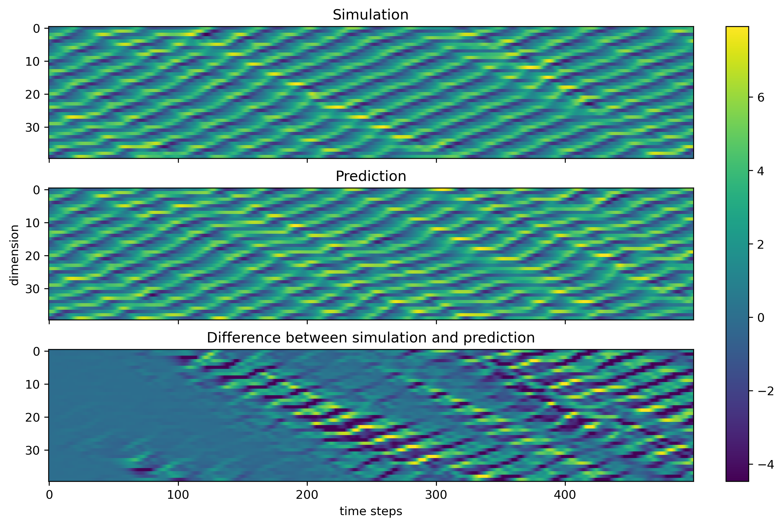
Plot the prediction results.

fig, axs = plt.subplots(3, 1, sharex="all", figsize=(9, 6),
                            constrained_layout=True, dpi=300)

vmin = np.min(y_test)
vmax = np.max(y_test)

im = axs[0].imshow(y_test.T, aspect='auto', vmin=vmin, vmax=vmax)
axs[0].set_title("Simulation")

axs[1].imshow(y_pred.T, aspect='auto', vmin=vmin, vmax=vmax)
axs[1].set_title("Prediction")

axs[2].imshow(y_pred.T - y_test.T, aspect='auto', vmin=vmin, vmax=vmax)
axs[2].set_title("Difference between simulation and prediction")

axs[1].set_ylabel("dimension")
axs[2].set_xlabel("time steps")
fig.colorbar(im, ax=axs)
plt.show()