Simulations Example

Short usage example for the rescomp.simulations module. We only simulate/plot a small number of different systems here. All the other implemented systems are called analogously.

Import the packages

import rescomp
import numpy as np
import matplotlib.pyplot as plt
from mpl_toolkits import mplot3d

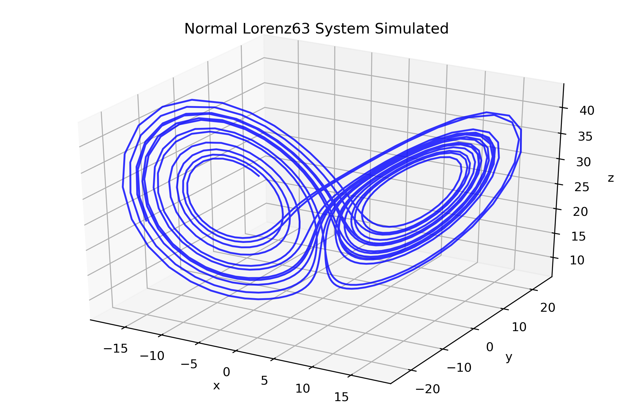
Simulate the normal Lorenz 63 System

simulation_time_steps = 1000
starting_point = np.array([-14.03020521, -20.88693127, 25.53545])

sim_data = rescomp.simulate_trajectory(
    sys_flag='lorenz', dt=2e-2, time_steps=simulation_time_steps,
    starting_point=starting_point)

Plot the normal Lorenz 63 System

fig = plt.figure(figsize=(9, 6), dpi=300)
ax = fig.add_subplot(111, projection='3d')
ax.plot(sim_data[:, 0], sim_data[:, 1], sim_data[:, 2],
        alpha=0.8, color='blue')

ax.set_title("Normal Lorenz63 System Simulated")
ax.set_xlabel('x')
ax.set_ylabel('y')
ax.set_zlabel('z')
plt.show()

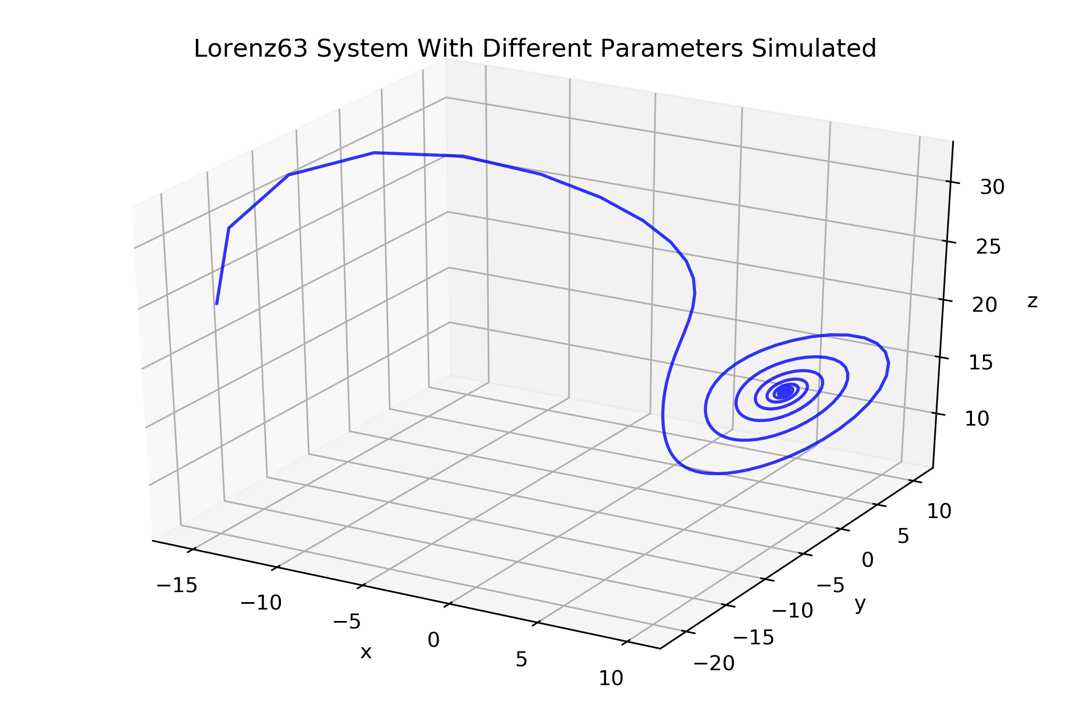
Simulate the Lorenz 63 System with parameters different than the default.

For more information on the possible parameters, please see the rescomp.simulations documentation

sigma=20  # default: sigma=10
rho=14  # default: rho=28
beta=8/3  # default: beta=8/3

sim_data = rescomp.simulate_trajectory(
    sys_flag='lorenz', dt=2e-2, time_steps=simulation_time_steps,
    starting_point=starting_point, sigma=sigma, rho=rho, beta=beta)

Plot the Lorenz 63 with different parameters

fig = plt.figure(figsize=(9, 6), dpi=300)
ax = fig.add_subplot(111, projection='3d')
ax.plot(sim_data[:, 0], sim_data[:, 1], sim_data[:, 2],
        alpha=0.8, color='blue')

ax.set_title("Lorenz63 System With Different Parameters Simulated")
ax.set_xlabel('x')
ax.set_ylabel('y')
ax.set_zlabel('z')
plt.show()

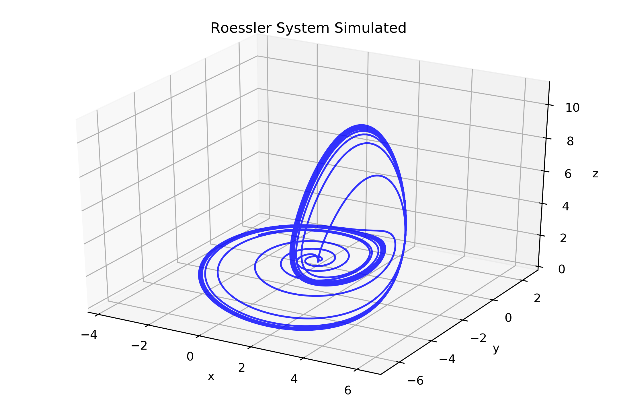
To simulate the Roessler System instead, just change the sys_flag parameter

simulation_time_steps = 5000
starting_point = np.array([0, 0, 0])

sim_data = rescomp.simulate_trajectory(
    sys_flag='roessler', dt=2e-2, time_steps=simulation_time_steps,
    starting_point=starting_point)

Plot the Roessler System

fig = plt.figure(figsize=(9, 6), dpi=300)
ax = fig.add_subplot(111, projection='3d')
ax.plot(sim_data[:, 0], sim_data[:, 1], sim_data[:, 2],
        alpha=0.8, color='blue')

ax.set_title("Roessler System Simulated")
ax.set_xlabel('x')
ax.set_ylabel('y')
ax.set_zlabel('z')
plt.show()